IS-LM Model
integrates real (Iinvestment Savings: IS) with money (Liquidity
Money: LM).
IS: (Investment - Savings:REAL)
Variables:
- Y real GDP
- C consumption
- I investment
- G government expenditures
- T taxes
- i interest rate
- a, b , I0 ,and c known constants
Equations
Note: Equation 3 is the investment function which says
that the higher the rate of interest the more attractive are risk
free government securities versus risky private investments. Thus
the amount of private investment decreases as the interest rate
increases. To invest in a private project, the rate of return must
equal the market interest rate plus a premium for the higher risk.
LM: (Liquidity - Money: Money)
Variables:
- Md demand for money
- Ms supply of money
- p price level
- Md/p real demand for money;
Ms/p real supply of money
- e,f are known constants
Equations:
Note: Equation (4) is the Keynesian money market equilibrium
equation. The first term on the right of (5) is the transactions
demand for money and the second term is the speculative demand for
money. Individuals hold a portfolio of assets such as money, stocks,
bonds, real estate, etc. The individual holds money in the portfolio
to take advantage of opportunities which may present themselves. As
the interest rate rises the opportunity cost of holding money
increases and he or she shifts from money to other assets.
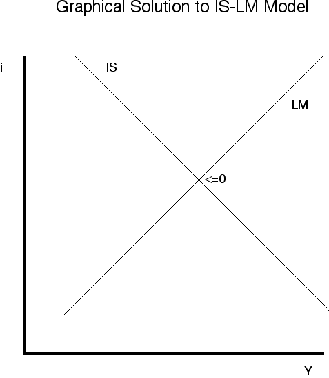
Solution to the IS-LM model
How to solve the IS model is in the notes. The IS curve is:
where k = 1/(1 - b) and A = a + I0
+ G - bT Important terms
The LM curve is obtained by substituting (4) into (5) to obtain:
To obtain the solution to the entire model rewrite (6) and (7) as
Note: (6') and (7') are 2 equations in Y and i that can be solved by
High School algebra. [Pain in the ass] Note: (6'==IS)
contains fiscal policy G and T and (7'==LM) contains monetary policy Ms. See
1st graph below. Remember IS slopes down to right while LM slopes up to right.
Solution to IS-LM Model
Equilibrium Graph
Example: Given G = 200; T = 150; Ms = 100; p = 1.0; a = 100;
b = 2/3; I0 = 600; c = 2500; e = 0.25; and
f = 1250 which implies K = 6/5 or 1.2 Note: K
= k/[1 + (ekc/f)]; A = a + I0
+ G - bT
What is the equilibrium Y? Use (8), definition for A and
value given for K
Y = 1.2(100 + 600 + 200 - 100 + (2500/1250)100) = 1200
and we can derive the following D equations:
Fiscal Policy
| DY
= KDG and DY
= -bKDT (9) |
|
Note: For the first fiscal model for exam 1, we had
D equations for Da and DI. For this model there are similar equations for Da and DI0. If you are an A student, if is in your
interests to figure out what these equations are? Do the involve K or k, that
is the question.
Fiscal Policy Graph
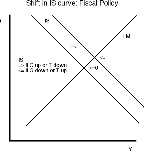
Let us assume you are hungry for a big A, then you should conisder
how Da and DI0 affect the solution. Do they affect the
IS or the LM curve and how? Suppose to reduce unemployment the government
desire to raise Y by 48 what is the required DG?
Use DY = KDG hence 48 = 1.2DG or DG = 40
Crowding Out: Impact on Private Investment
In the graph above increasing G or decreasing T raises the interest
rate and this affect the level of private investment.
DI = -cDi. Equation (10) above is obtained by manipulation to obtain DI as a function of DY. If G is increased by the amount in b above, how much I is crowded out (Assuming
p remains constant)? We use formula DI = -(ce/f)DY ABOVE that was derived in the notes. DI = -(2500(.25)/1250)48 = -24
Monetary Policy Graph
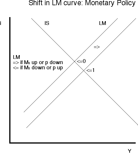
Suppose p starts increasing due to either cost push (OPEC) or
demand pull (Viet Nahm) war. The LM curve starts moving to the left and the
interest rate starts rising. The head of the Fed knows that expanding the
money supply under such conditions is like throwing gasoline on a fire, so
why does he( someday she) do so. Once interest rates go above 20% there is
a risk that many many businesses will go bankrupt and cause a major recession,
if not a depression. Therefore expanding the money supply is the lessor of
two evils.
Compensating Monetary Policy
| D(Ms/p)
= |
f
Kc
|
(k -K) DG (11) |
|
Ideal Fiscal with Accomodating Monetary Policy
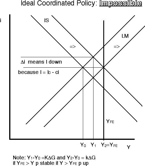
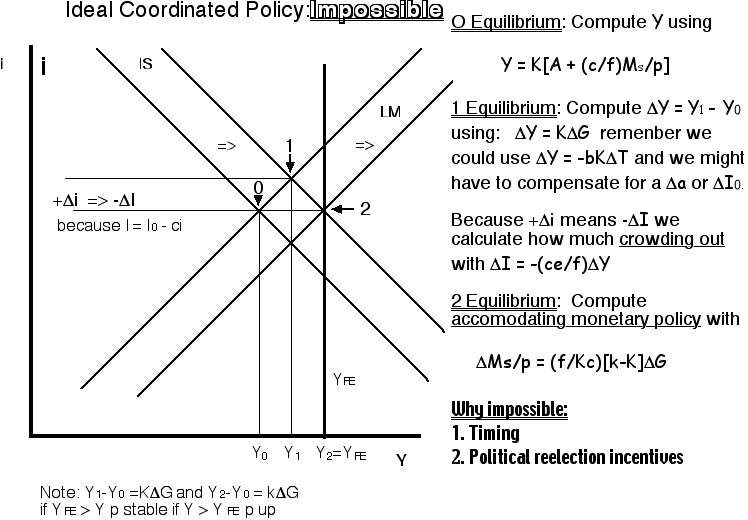
IV. Now suppose the real money supply Ms/p is increased to compensate the
crowding out. What is DMs/p? We use D(Ms/p) = [f/ Kc](k -K) DG to obtain DMs/p = 30
Another problem for you to work out
IS:
- Y = C + I + G
- C = a + b(Y - T)
- I = I0 - ci
LM:
Variables:
- Y real GDP
- C consumption
- I investment
- G government expenditures
- T taxes
- i interest rate
- Ms is the money supply
- p is the price level
- i is the interest rate
- a, b, c, e, f, and I0 are known constants
The solution to the IS model is:
- Y = k(A - ci)
- k = 1/(1-b)
- A = a+I0+G-bT
The solution to the IS-LM model is:
Change equations:
- DY = KDG
- DI = -(ce/f)DY
- D(Ms/p) = [f/ Kc](k -K) DG
Given
- G = 1000
- T = 1000
- Ms = 400
- p = 2
- a = 150
- b = 2/3 You must know how to figure out k
- I0 = 300
- c = 2500
- e = 0.25
- f = 1250
- K = 1.2
- Why is K < k? Explain either mathematically or economically? Is denominator
greater than 1? Economically: Think crowding out!
- What is the equilibrium Y? Which equation do you use?
- To reduce unemployment the government desires to raise Y by 108. What is
the required DG? What is an alternative fiscal instrument which could be used to achieve the
same objective? What about DT? Remember with
DT the change equation is slightly different than
for DG?
- How much investment is crowded out? Which change equation do you use?
- Now suppose the real money supply Ms/p is increased to compensate the crowding
out. What is DMs/p? Again, which change equation do you use?
- Suppose Y before increasing G is less than the full employment Y. If increasing
G increases Y beyond the full employment Y what will happen? Will p remain
stable?
- Return to part III above. What is the required DG if at the same time DI0 is -10. How does this affect the rest of
the problem?
File translated from TEX by TTH,
version 2.25.
On 31 Oct 1999, 11:27.
Revised: Tuesday, 6 Nov 01