Consumer Theory

In this section we shall provide a simple calculus version of consumer theory. The standard calculus approach to consumer theory involves using Lagrangian multipliers. Since our objective is only to use one variable calculus, we shall solve the two variable consumer problem by substitution to reduce the number of variables to one.

Budget Constraint

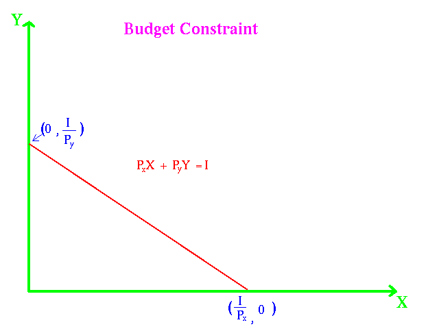
In the marketplace the typical household buys a large number of products. To represent a large number of products is beyond the scope of the course. We shall limit ourselves to two goods

x and

y. The price of

x is

p_x and the price of

y is

p_y. The student should recognize that

p_x,

y, and

p_y are variables which can take on any values. The amount the consumer spends on

x is

p_x

x and the amount spent on

y is

p_y

y. The consumer in the period under consideration, (hour, day, week, quarter, or year), has and income

I. We assume that the consumer always spends all his or her income on some combination of

x and

y. Therefore, the consumer has a budget constraint:

_____p_xx + p_yy = I _______________ (1)

A graph of the budget constraint is shown below:

Utility Function

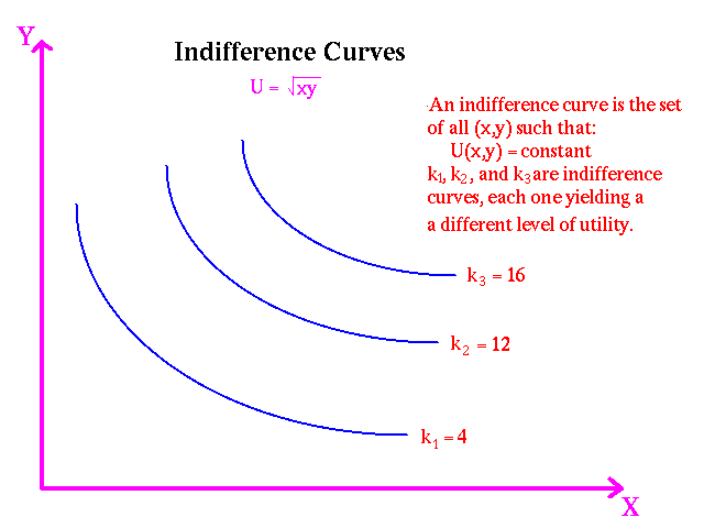
Each consumer is assumed to have a utility function which represents his or her tastes concerning alternative combinations of goods,

U(x,y). For example,

U(3,4) = 10,

U(4, 5) = 12 , and

U(4, 3) = 10. For the utility functions used in this course there is no satiation, that is

z > 0 => U(x + z,y) > U(x,y) and z > 0 => U(x,y + z) > U(x,y) .

That is more is better than less. An indifference curve of a utility function is the line representing all combinations of x and y which result in the same value of the utility function. In the example above the points (3,4) and (4,3) lie on the same indifference curve. To keep the calculus as simple as possible we shall use concave utility functions. Concave utility functions have indifference curves of the following form:

Optimization Model

The consumer problem is:

_____max U(x,y)
_____subject to p_xx + p_yy = I _____________ (2)

In words, the consumer compares alternatives bundles and chooses the one which has the highest utility. We do not ask how the consumer performs this operation, but rather we examine the consequences of such action which we will soon see results in demand functions for x

To solve this problem by substitution let us consider a specific concave utility function: U(x,y) = x^1/2y^1/2

Deriving the Consumer's Demand Curves

We shall consider three examples of about the degree of difficulty that you will encounter on tests.

Example I:

The first example is:

_____max x^1/2y^1/2

_____subject to p_xx + p_yy = I ____________ (3)

We use the budget constraint to determine:

_____y = (1/p_y)[I - p_xx ]________________ (4)

We substitute (4) into the utility function to obtain:

_____f(x) = x^1/2[(1/p_y)(I - p_xx)]^1/2________ (5)

The optimization problem has been reduced to one variable x:

_____maxf(x) = x^1/2[(1/p_y)(I - p_xx)]^1/2_____ (6)

We take the first derivative using the product rule:

_____f'(x) = (1/2)x^-1/2[(1/p_y)(I - p_xx)]^1/2 + (1/2)x^1/2[(1/p_y)
__________ (I - p_xx)]^-1/2(-p_x/p_y)____________ (7)

We set f'(x) = 0 and obtain:

_____ (1/2)[(1/p_y)(I - p_xx)]^1/2/[x^1/2] = (p_x/2p_y)x^1/2/[(1/p_y)
_______________________________ (I - p_xx)]^1/2__ (8)

Multiplying both sides by the denominators we obtain:

_____ (I - p_xx) = p_xx_____________________ (9)

Solving for x, we obtain:

_____ x = I/2p_x_________________________ (10)

From the budget constraint, we obtain the demand curve for y:

_____ y = I/2p_y_________________________ (11)

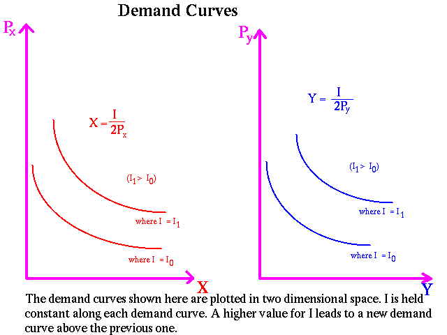
We have obtained the demand curve for x and yas functions of the income, I and price of x, p_x. Now when we draw a graph, we do so in two dimensions. But we have three variables. The two dimensional demand curve is drawn showing x as a function of p_x holding I constant. We obtain a family of demand curves, one for each value of I.

Again the two dimensional demand curve for y shows the relationship between y and p_y. The shift parameter is I. It is important to understand the difference between a movement along a demand curve (relationship between y and p_y holding I constant) and a shift in a demand curve (the consequences in the value of I). The family of demand curves for x and y are shown below:

Example II:

The second example is:

_____max x^2/5y^3/7

_____subject to p_xx + p_yy = I _______________ (12)

We use the budget constraint to determine:

_____y = (1/p_y)[I - p_xx ]___________________ (13)

We substitute (13) into the utility function to obtain the following optimization problem:

_____maxf(x) = x^2/5[(1/p_y)(I - p_xx)]^3/7________ (14)

We take the first derivative using the product rule:

_____f'(x) = (2/5)x^-3/5[(1/p_y) (I - p_xx)]^3/7 + (3/7)x^2/5[(1/p_y)
___________(I - p_xx)]^-4/7(-p_x/p_y)____________ (15)

We set f'(x) = 0 and obtain:

_____ (2/5)[(1/p_y)(I - p_xx)]^3/7/[x^3/5] = (3p_x/7p_y)x^2/5/[(1/p_y)
_______________________________ (I - p_xx)]^4/7__ (16)

Multiplying both sides by the denominators we obtain:

_____ (2/5)(I - p_xx)] = (3p_x/7)x_____________ (17)

Solving for x, we obtain the demand curve for x:

_____ x = 14I/29p_x_______________________ (18)

From the budget constraint, we obtain the demand curve for y:

_____ y = 15I/29p_y_______________________ (19)

The graphs of the families of demand curves for the two variables are similar to those shown above for example I. The degrees of difficulty of this example corresponds to a B level of performance.

Example III:

The third example is:

_____max x^1/2 + y^1/2

_____subject to p_xx + p_yy = I ________________ (20)

We use the budget constraint to determine:

_____y = (1/p_y)[I - p_xx ]____________________ (21)

We substitute (21) into the utility function to obtain the following optimization problem:

_____maxf(x) = x^1/2 + [(1/p_y)(I - p_xx)]^1/2_______ (22)

We take the first derivative using the product rule:

_____f'(x) = 1/(2x^1/2) - p_x/2p_y[(1/p_y)(I - p_xx)]^1/2_ (23)

We set f'(x) = 0 and multiplying both sides by the denominators we obtain:

_____ [(I - p_xx)(py)] = p_x²x___________________ (25)

Solving for x, we obtain the demand curve for x:

_____ x = Ip_y/[p_xp_y + p_x2]_____ (16)

From the budget constraint, we obtain the demand curve for y:

_____ y = Ip_x/[p_xp_y + p_y2_____ (19)

The graphs of the families of demand curves for the two variables have two shift parameters: Income and the price of the other good. In a model with many goods the prices of a subset of the goods would be shift parameters.

Ordinal Utility Functions

If in example I we replace the utility function

U(x,y) = x^1/2y^1/2 with

U(x,y) = 2x^1/2y^1/2, what will be the affect on the derivation of the demand curves. If you examine the derivation closely, you will see that the factor of 2 will cancel out and the demand curves will be unchanged. The same is true if will multiply the utility function by 3 of any other constant. (Indeed, the demand curves are invariant to any monotonic transformation). What this means is that there is not one but a family of utility functions which will derive a particular set of demand curves. The utility function is ordinal because we are not interested in the magnitude of the utility number in ranking two alternative bundles, but simply which number is larger.

Quiz

Index