Optimization Theory

Introduction

In this section we will consider two optimization models. The first is a discrete model and the second is a one variable calculus model. The purpose of using two models is to show that the economic implications are a function of what type of mathematical model is assumed.

Discrete Model

We wish to find the maximum

f^*(i) of a set

{f(i): i = 1,2, ... ,n}. To find the maximum we must perform a search through every element of the set as follows:

Step 1: Is the first element bigger than the second? If so the first element is the temporary maximum. If not, the second element is the temporary maximum.
Step 2: Is the next element bigger than the temporary maximum. If so, the next element becomes the temporary maximum.
Step 3: Repeat step 2 until the nth element in the set has been checked. The maximum is the temporary maximum.

Note than with a discrete set, the search for a maximum requires us to examine every element in the set to find a maximum. Let Þ(i) = f(i + 1) - f(i) and suppose the set has the condition, monotonically decreasing difference, that Þ(i) > Þ(i+1) for i = 1,2, ... n-2 In this case there is a necessary condition for f^*(i) namely that Þ(i-1) > 0 and þ(i) < 0 or Þ(n-1) > 0. What this means in our search above is that we can quit the first time the new element is not made the temporary maximum.

Differentiable Function

The definition that

x^* is a local maximum of

f(x) in a neighborhood of

x^* is:

f(x^*) > or = f(x) for all in a neighborhood of x^*

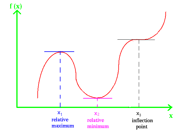
The definition does not provide an easy means of finding a relative maximum because we would have to examine an uncountable number of points to check out the definition. A necessary condition which enables to focus our search for relative maxima is intuitively obvious by examining the graph of f(x) shown below:

If you will examine the picture you will see that at the relative maximum at x^* that the tangent to f(x) is parallel to the x axis. This means that the slope of the tangent is equal to 0 at x^*. But, because the slope equals f'(x), a necessary condition that f(x^*) be a relative maximum is that f'(x^*) = 0

This necessary condition provides us with a condition that we can use to search for relative maxima.

Step 1: Determine f'(x)
Step 2: Set f'(x) = 0 and solve for x^*

Now let us consider two cases

1. f(x) = 1 + 2x - x²
2. f(x) = 1 - 2x + x²

Apply the two steps:

1. f'(x) = 2 - 2x
_ f'(x) = = 0 = 2 - 2x or
_ x^* = 1

2. f'(x) = -2 = 2x
_ f'(x) = = 0 = -2 + 2x or
_ x^* = 1

However, if we look at the graphs of the two functions we can see that the first case is a relative maximum and the second case is a relative minimum.

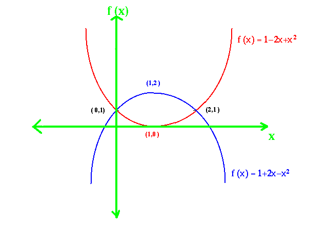The problem is that is the only condition we use is f'(x^*) = 0 to search for x^* we will find relative maxima, relative minima as well as inflection points. We need a stronger condition to separate these three cases.

Since this is a freshman course, we will use a condition which will greatly simplify the problem. The type of functions we shall consider in this course will all have the property of concavity.

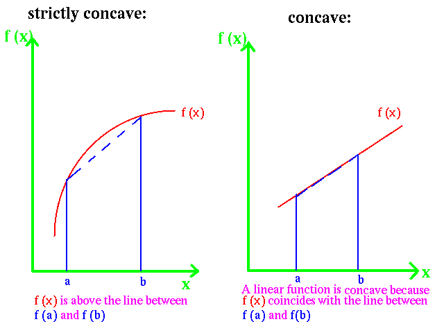
Definition: f(x) is concave over its domain if for any two points x₁ and x₂ in its domain,
f((1-c)x₁ + cx₂) > or = (1-c)f(x₁) + cf(x₂) where 0 < c < 1 Two graphs of concave functions are shown. The first case is > ( strictly concave) and the second case with linear segments is =.

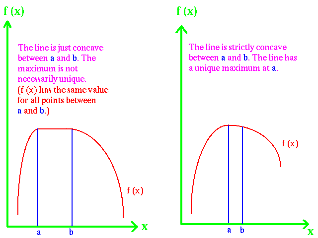
What simplification does concavity give us? With concavity the necessary condition f'(x) = 0 becomes both necessary and sufficient that an x^* which satisfies f'(x^*) = 0 is a global (not relative) maximum. With concavity there can only be one global maximum. If f(x) = 0 is strictly concave, the maximum is unique. If f(x) = 0 is just concave, the maximum is not necessarily unique. See graph below:

Sample Problems:

1. f(x) = x^(3/4) - x

_ f'(x) = (3/4)x^-(1/4) - 1

_ f'(x) = 0 or 3/[4x^(1/4) = 1

_ x^(1/4) = 3/4

_Now remember that xⁿx^m = x^n+m and (xⁿ)^m = x^nm

_Therefore we raise each side to the power of 4.

_(x^(1/4))⁴ = (3/4)⁴

_or x = (3/4)⁴

2. f(x) = x^(1/3) - x

_ f'(x) = (1/3)x^-(2/3) - 1

_ f'(x) = 0 or 1/[3x^(2/3) = 1

_ x^(2/3) = 1/3

_We raise each side to the power of (3/2).

_(x^(2/3)^(3/2) = (1/3)^(3/2) or x = (1/3)^(3/2)

Optimization with a linear constraint

Consider the following optimization problem: Find (x^*,y^*) which maximize f(x,y) subject to the constraint that x + y = 1. We shall solve this problem by substitution which reduces the optimization problem to one dimension.

From the constraint we obtain y = 1 -x and we substitute this relationship into f to obtain g(x) = f(x, 1-x). We can then optimize g(x) to obtain x^* and obtain y^* = 1 - x^*.